Practical Feature Selection for Algorithmic Trading

An Unconventional Approach

This is a slightly strange approach to choosing the right features for algorithmic trading that is expensive but has worked well for me and seems to provide a very well balanced and all encompassing set of features for use in the ML algorithm of choice.

The following was a happy tangent, and interesting detour while doing some research for a master’s project on the subject.

While considering suitable trading indicators and engineered features to apply to my autonomous trading bot, I decided to, approach this problem as if seeing it for the first time, despite having some prior knowledge of the subject. The aim was to try and get the largest bang for my buck, the most information condensed into the least amount of features.

Engineering Features

Starting where most do, with the Open, High, Low, Close, Volume data, I then proceeded to build up some few features;

I decided first to convert the timestamp information into a cyclical encoded variable. Using the minute in the hour, hour in the day, etc. I made sure that each of the parts could be represented as a float.

# timestamp encoder

def cyclical_time_encoding(df):

    # Apply cyclical encoding using sine and cosine functions
    df['year'] = (df['timestamp'].dt.year - 1980 )/ 200
    df['month'] = df['timestamp'].dt.month / 12
    df['day'] = df['timestamp'].dt.dayofyear / 365
    df['hour'] = df['timestamp'].dt.hour / 24
    df['minute'] = df['timestamp'].dt.minute / 60

    return df

 

Then, remembering that I am approaching this with a spirit of discovery, I wrote loops to create multiple versions of the same feature. For example, considering the moving average of the closing price, instead of setting it to one window, I looped over multiple windows and allowed the number of features to grow. For example:

 

import ta  # Import the ta library for moving average calculation

for window in range(5, 106, 20):
    # Generate the column name for the moving average
    column_name = f'sma_{window}'  
    # Calculate the simple moving average and store it in the dataframe
    df[column_name] = ta.trend.sma_indicator(close=df['close'], window=window)

 

A lot of the work behind building the features came down to using the python ta library. It is a fantastic library that is home to one of the most useful little functions I have ever seen; ta.add_all_ta_features(). This uses the basic OHLCV data to populate a data-frame with 100+ additional features.

The Search

For this project, I had downloaded a relatively large collection of data from the Alpaca trading platform:

• 3000+ Stock Histories
• 5 minute interval data
• 7 year window of observation
• ~32 GB of data prior to feature engineering

Usually when dealing with a single dataset, one can use any of a large list of techniques I felt that in this case a hybrid approach would be required. Stocks, like persons, have their own characters, and while some features may be useful with some, other features may be more useful with others. My aim was to find a set of features that would be relatively robust and applicable across most of the stock histories with some expectation of success.

My first thought was to try and use the correlation in order to remove the features with the largest mutual correlation. This works by calculating the correlation matrix between all of the features and the label. The couple of features which have the highest mutual correlation is selected and the feature out of the pair with the least correlation to the label is removed. These steps would then be repeated until some threshold is reached, such as ending up with the best 10 features. This would have worked fine were it not for the huge number of features produced in the prior step. The combinations produced through the large number of features would have been very hard to compute on my machine, too expensive on someone else’s and worst of all take up too much time before my deadlines.

Time for some lateral thinking.

I tried quite a few things before ending up at this solution, however I will spare myself the pain of having to re-live the embarrassing ideas and skip to the part that worked. I strongly urge the reader to imagine I got it right first try.

What worked, was to think of each stock as a separate entity and sample its feature set multiple times. The, correlation based, feature reduction process explained above, was used on much smaller samples reducing the computational load significantly, and by making sure to sample enough times the probability that all the pairs existed at least once in the groups was also reasonably high.

The surviving features for each run in each stock history were all then grouped together and their frequency used to determine their importance across all of the datasets.

A different way to think about this, would be to imagine each of the stock histories having 10 votes to allocate to 100 features, and instead they were given 5 votes to allocate to 7 samples of 20 features. Even as a person you can imagine choosing 5 from 20 a much easier task than trying to compare 100. Since they would have still compared most of the features to each other looking at the top 10 features with the highest votes will in most cases result in a very similar result. Taking into account that this test pulls together samples from over 3000 different stock histories, it’s safe to say that any quirky sampling glitches can be expected to fade away, thanks to the massive size of the sample set.

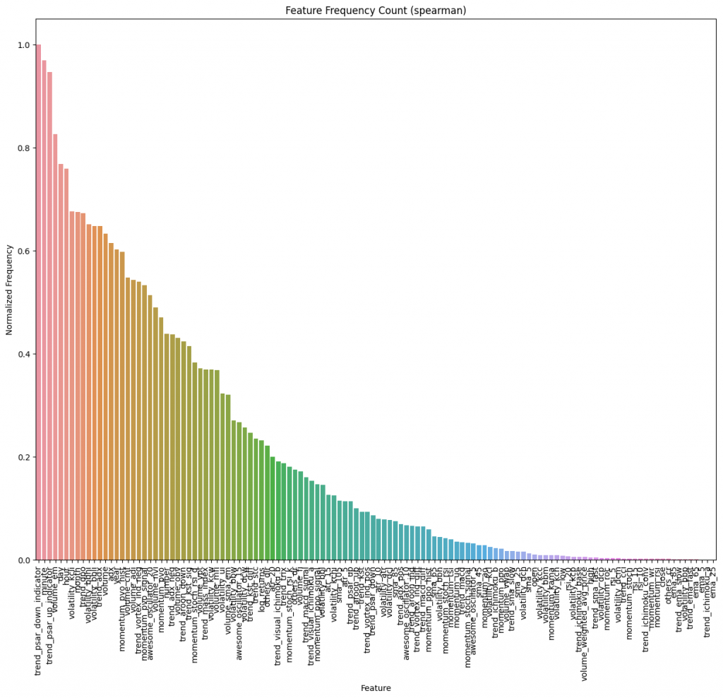
This is a histogram with the results acquired from performing the test over the entire corpus. In the end I kept it simple and chose the top 20% of features in order to leverage the Pareto principle and up with what would be expected to be the top performing feature set for predicting my label.